What is a sample?
The goal of inferential statistics is to make inferences (or estimates) about what’s happening in a population. We can’t usually ask everyone in a population to answer our survey, so we use a random sample from that population.
A random sample is always going to look a little bit different from the population from which it was drawn. In other words, there’s going to be a bit of sampling error between the average we might calculate for a population and the average we calculate for a sample. Based on the principles of a sampling distribution, we can estimate just how much error there might be in our estimates.
What is a sampling distribution?
A sampling distribution shows what would happen if we repeatedly drew random samples of the same size from the same population and calculated the same statistic each time. We don’t actually ever do this in real life, but knowing what would happen helps us make estimates about the one sample we do select.
Sampling distributions help us understand how much a sample statistic can vary simply because of random sampling. Some samples will produce means below the true population mean (μ) and some above it.
If we draw more and more random samples, we can see the theoretical sampling distribution more clearly. The theoretical mean of the sampling distribution of sample means () is equal to the population mean (). In our simulation, the mean of the sample means will get closer to as we add more samples.
Sampling Distribution Simulator
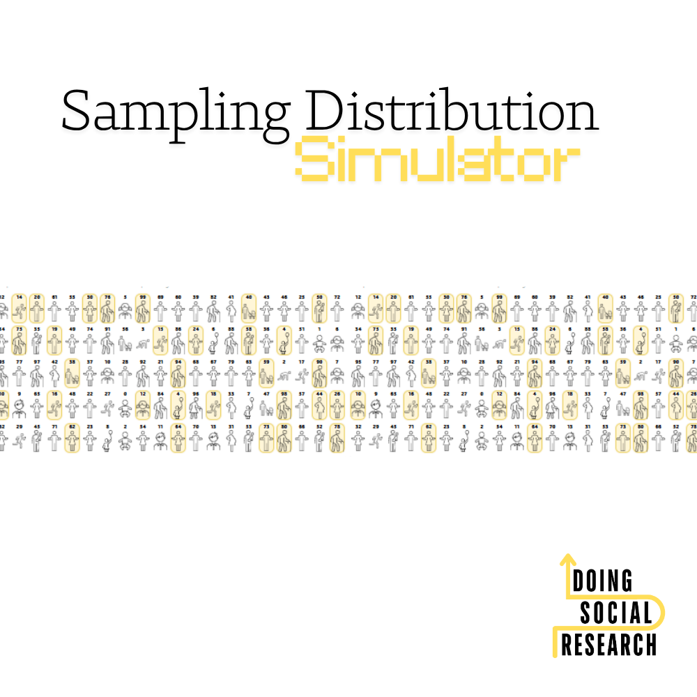
Below is a sampling distribution simulator that lets you see these ideas in action. The simulator begins with a population of 100 people who differ by their age. Because we can see the entire population, we know the true average age of everyone in the population (μ).
Choose a sample size (n) and draw a random sample from the population. The simulator will calculate the average age of the people in your sample (x̄). Notice which people were randomly selected and how the sample mean compares with the population mean.
Next, add your sample mean (x̄) to the sampling distribution. The x̄ that appears on the graph represents the mean from that one random sample. Draw another sample and add its mean. As you repeat this process, you will see a sampling distribution of means begin to take shape. You can then use the +1, +10, +50, and +100 buttons to speed things up.
Try changing the sample size (n) and starting again. Compare the sampling distribution for a very small sample (n = 3) with those for larger samples (n = 10, 30, or 50). What happens to the shape and spread of the sampling distribution? How closely do the sample means cluster around the population mean (μ)?


What’s the Central Limit Theorem?
The Central Limit Theorem tells us what happens to the sampling distribution of the mean as we increase the size of each random sample (n). As sample size increases, the sampling distribution will:
- become increasingly close to the shape of a normal distribution, even when the original population is not normally distributed;
- become less spread out and have a smaller standard deviation (the standard deviation of a sampling distribution is called the standard error or σx̄); and
- remain centred around the population mean (μ).
This means that larger samples tend to produce more precise estimates of population parameters—that is, estimates with less sampling error.
(Note: σ is the Greek letter sigma and μ is the Greek letter mu. We conventionally use Greek letters to represent population parameters—the values we are usually trying to estimate but cannot observe directly. We use Roman letters for the equivalent sample statistics: s for the sample standard deviation and x̄ (“x-bar”) for the sample mean.)
What do we use this for?
This is all mostly theoretical at this point, but we will use these principles to estimate how much sampling error is associated with our statistics when we calculate things like confidence intervals, t-tests, and the statistical significance of regression coefficients.
See also: Samples vs. Populations