Chi-Square in SPSS

Last updated on December 6, 2021

Chi-Square in SPSS

Calculating a chi-square statistic in SPSS is quite simple, as long as you have two categorical variables. The much harder part is in the interpretation (which we’ll get to way down below). In the example here, we are using 2016 Census (Canada) data with the following variables:

• School Attendance, asked in the survey as “At any time since September 2015, has this person attended a school, college, CEGEP, or university?” with the following possible responses:
  1. Did not attend school
  2. Elementary or secondary school
  3. Technical or trade school, community college or CEGEP
  4. University
  5. Multiple responses
• Bedrooms, asked as “number of rooms in a private dwelling that are designed mainly for sleeping purposes even if they are now used for other purposes.” One could probably treat this as an interval ratio variable but there are few possible categories and the variable is top-coded making it more ordinal, so it is acceptable to use for a chi-square. The responses are coded as follows:
  • 0=no bedroom
  • 1=1 bedroom
  • 2=2 bedrooms
  • 3=3 bedrooms
  • 4=4 bedrooms
  • 5=5 bedrooms or more

Before running any analyses, always be sure to recode your variables, renaming them and making sure that all missing data are coded out (although I didn’t do that here. Do as I say, not as I do.) Once your variables are read for analysis, the chi-square steps are pretty easy.

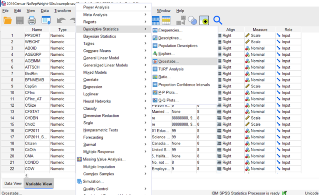
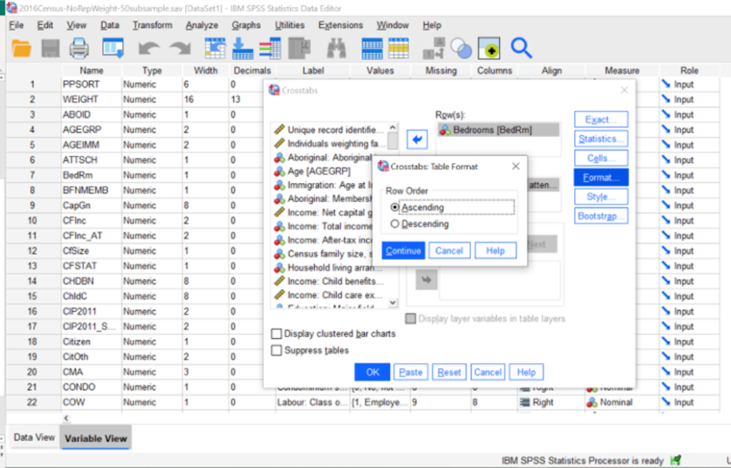
1. Click on Analyze –> descriptive statistics –> Crosstabs…

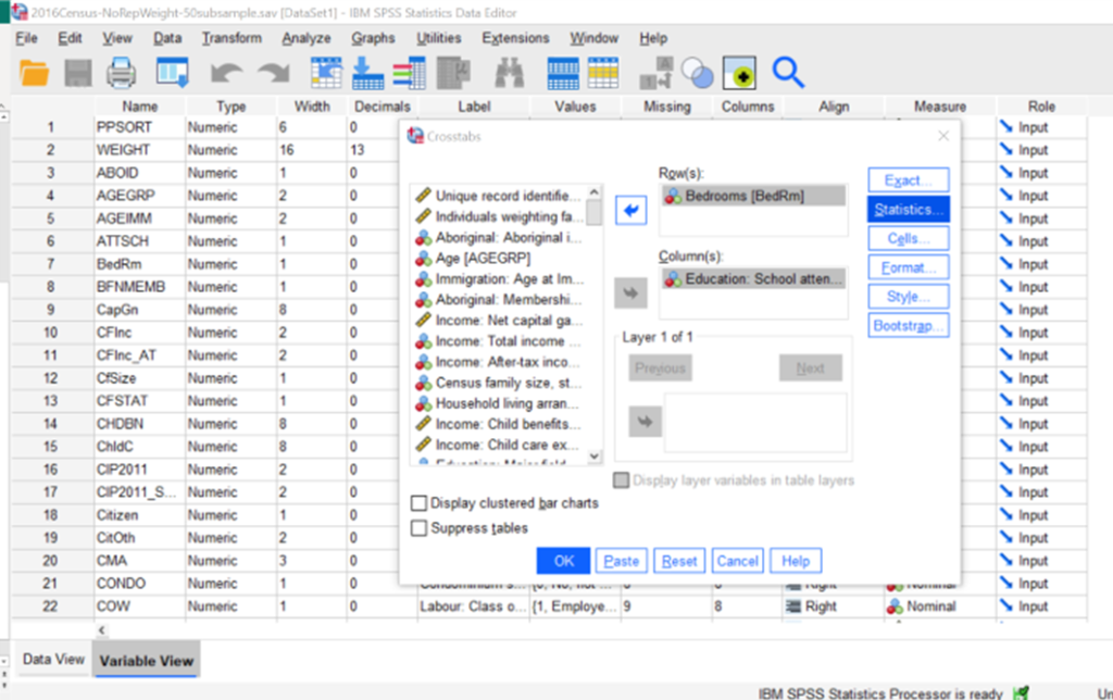
2. The main crosstabs screen will pop up. For this example, we’re going to put our independent variable (Education) in the columns, and the dependent variable in the rows (bedrooms). Then click on the button for Statistics (in blue on the right in my example image below).

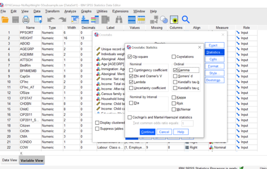
After clicking statistics, you get a screen with the various statistics you can ask SPSS to calculate for you. You’ll definitely want to click chi-square if you want to calculate a chi-square, but you may want other statistics such as the proportional reduction in error (PRE) tests like Lambda or Gamma, or a measure of association like Phi and Cramer’s V. Those are the only ones students in my course (SOC 3142) will need, but selecting which one will always depend on the level of measurement of the variables. After ticking the boxes for the stats you want, click Continue.

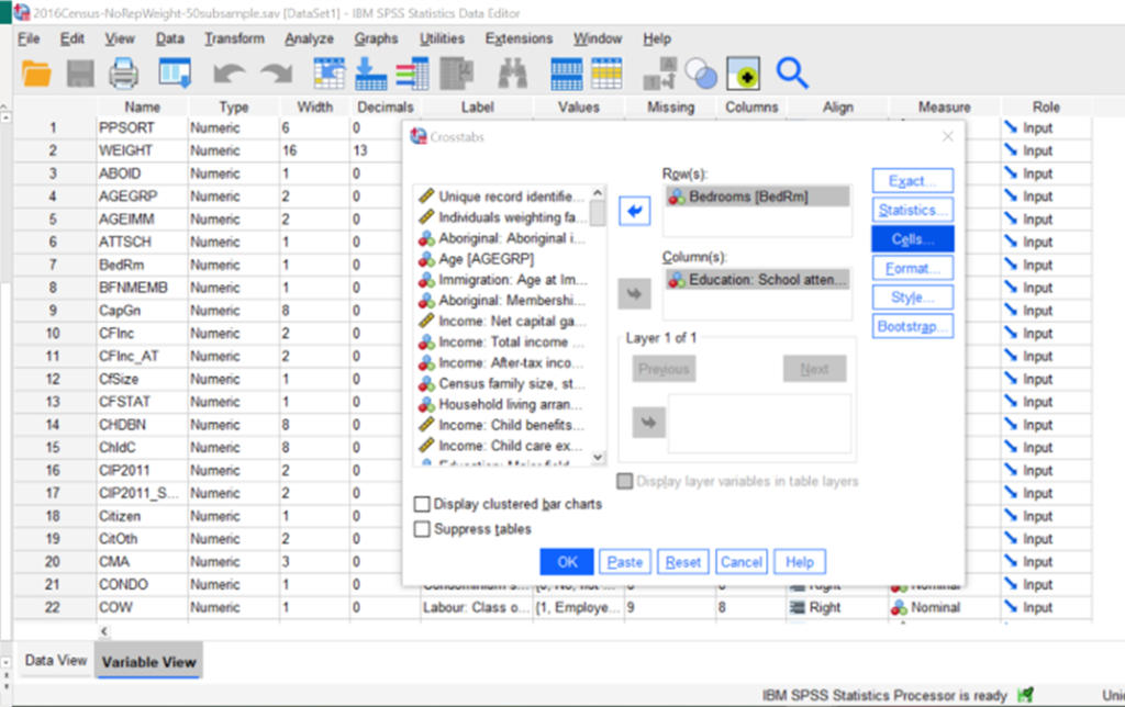
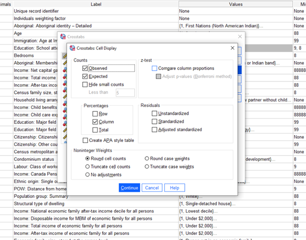
Back at the main crosstabs screen, click on Cells… in order to get SPSS to calculate percentages for your table.

Because we put our independent variable (IV) in the columns, and our dependent variable (DV) in the rows, we want SPSS to calculate percentages going down the column. (If you switched your IV & DV, you would calculate percentages for the row.) We want the observed frequencies for interpretation, but we almost might include the expected frequencies to make sure they are all greater than 5 (the chi-square test won’t work if the expected frequencies are less than 5). You could do a z-test to compare column proportions (not something I did in my class), and you can ignore the residuals options for now. Click continue.

If you want to change whether the rows go from low to high values (1, 2, 3, 4, 5) or high to low values (5, 4, 3, 2, 1), go into format and select either ascending (low to high) or descending (high to low). Click continue. Then click OK on the main Crosstabs screen.

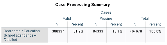
The output that you get will begin with a case processing summary. This is useful if you want to know your sample size and how much missing data you have, but not much else. Moving on…

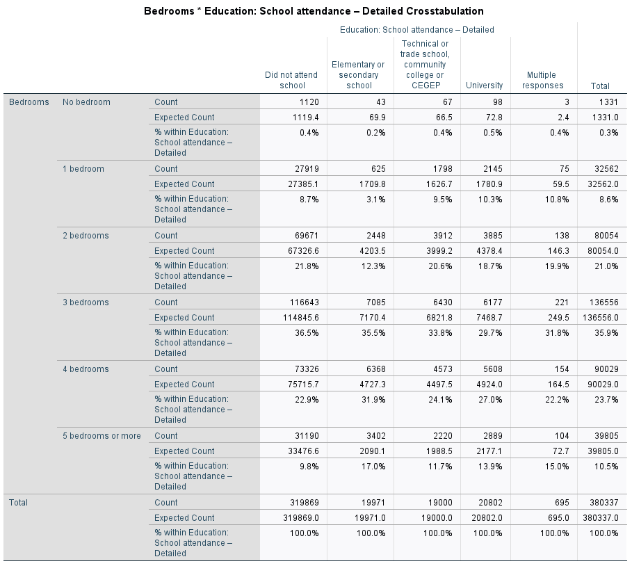
The next block is the meat of the story. This is the crosstab table, where you can see the observed frequencies and the percentages by column. Notice that one of the cells (Multiple responses and no bedroom) had an expected value of only 3! This won’t work, so we need to collapse the categories or remove those people.

Deciding what to do can be tricky and you always should consider both theoretical and empirical reasons for what you do.

• Theoretical Reasons: If my research question really needs to include a particular category, I might want to make sure I don’t muddy the waters by combining two groups that don’t make sense to combine. For example, I probably would not want to combine “Multiple Responses” with “Did not attend school” unless I was interested primarily in people who attended only one school. If I don’t really care about the “Multiple responses” folks, I could recode them as missing, and basically just remove them from the analysis.
• Empirical Reasons: However, if I do that, my sample size will drop a lot. In the case of a Census where I’m working with almost 400,000 cases, the loss of 695 probably won’t have a big impact on our results. But in smaller samples, this could be a big deal. Generally speaking, the more missing data we have, the less we can trust that our sample speaks for the population from which it was drawn (and speaking for the population is the main reason why we go through the bother of calculating inferential statistics!).

I think the best solution in this case, so as not to lose cases, is to combine categories on the dependent variable. So, instead of having all the values of the number of bedrooms, I’m going to collapse them into three groups: Few bedrooms, average bedrooms, and lots of bedrooms. I’ll decide who belongs where by looking at the last column in the table with the total percentage of respondents who fall into each of the bedroom categories. What I see is that about a third of respondents (0.3% + 8.6% + 21.6%= 30.5%) have zero, 1, or 2 bedrooms; about a third (35.9%) have 3 bedrooms; and the remaining third (23.7% + 10.5%) have 4 or more bedrooms. I’ll recode the variable so that these will be my new categories, and then rerun all the steps again, to get the following table.

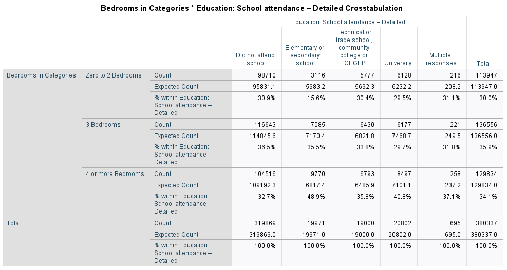
That’s much better! All of our expected counts are well over 5 and we can go on to interpreting our results. First thing to do is simply explore the numbers in the table. What differences do you see? Are there some groups that have a bigger difference in the number of bedrooms that they have than other groups? When the IV and DV are set up this way (columns and row, respectively) and we have calculated the percentages going down the columns, you want to compare moving across the rows. For example, let’s start with the zero to 2 bedroom folks, the largest group is “did not attend school in the past 5 years” and the smallest group is “elementary or secondary school.” Specifically, 15.6% of those who attended an elementary or secondary school and 30.9% of those who did not attend any school in the past 5 years live in a residence with zero to 2 bedrooms. Just eyeballing it, that looks like a pretty big difference, since the latter group is twice as big as the former. Looking at the other rows, there are fewer big differences among those in an average sized place with 3 bedrooms. The largest group is those who did not attend school (36.5%) compared to those who recently attended university (29.7%), a 6.8% raw difference. Finally, those who recently attended elementary or secondary school are the most likely to be found in a big house with 4 or more bedrooms (48.9%), compared to those who did not attend school recently (32.7%).

Given that this example is kind of boring (my apologies), deriving a lot of meaning from this example is a bit tricky. We also want to be careful not to overinterpret our results. Still, what I’m seeing so far in these numbers is that people who have recently attended elementary or secondary school live in bigger houses than those who have not attended school in the past 5 years. This makes sense to me, since those who recently attended elementary or secondary school are likely younger than average and live in families who would have homes with more bedrooms in order to fit the kids. Those who have not attended any school in the last 5 years are likely older, maybe their kids have left the nest, so they live in a smaller place. We can’t know any of this with any certainty, so again, don’t overinterpret the results to make grand conclusions, but looking at these results there isn’t some glaringly weird result that would make us question our results.

These results are all based on our sample alone, which is why we need the chi-square to make inferences about the population. In the case of chi-square we are testing the hypothesis that the the two variables (bedrooms and type of school attended in the past 5 years) are independent in the population. In other words, our null hypothesis is that these two variables have nothing to do with each other. To get the answer to that question, we look at the Chi-Square Tests output:

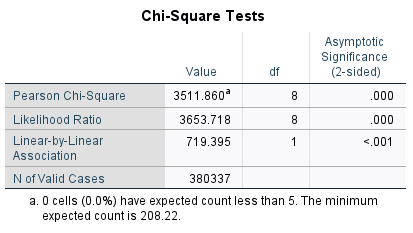
Note that 0% of the cells have expected counts less than 5! That’s because we did a good job fixing our first job. The Pearson Chi-Square value is what we are interested in, which here is 3,511.860 with 8 degrees of freedom. (Degrees of freedom is calculated based on the number of cells in the table: df=(number of rows -1)*(number of columns-1)=(3-1)*(5-1)=(2*4)=8. If we wanted to go old school, we could look at a chi-square table to see if we reach significance, but as modern folks, we can also just look at the column for significance. That shows us that this chi-square value does, in fact, surprise the critical value for p<0.001 and we can reject the null hypothesis. In other words, previous school attended and number of bedrooms are not independent; rather, they have a relationship with each other. This is why we saw that some of the categories had higher bedrooms than others.

However, remember when I said this is a boring example. It’s not just a boring example, it’s also kind of a weird example. I mean, why would we care about these two variables? What’s the theoretical reason for seeing if there is a relationship between these two variables? Is there really anything important in this relationship? Might not other factors, like, I dunno, income?!? have a bigger impact on how many bedrooms you have in your house? I would guess that whether you attended one or the other type of school is probably pretty UNimportant in the grand scheme of why someone ends up with a big house full of bedrooms. So, let’s look at some measures of association to see how important this relationship is.

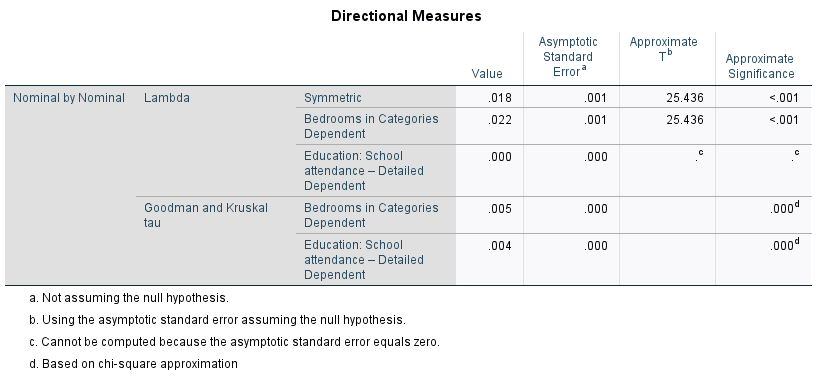
The first measure we’re going to interpret is the PRE statistic called Lambda. This is a directional measure, meaning that identifying which is the IV and which is the DV is important. In our example, bedrooms is our DV, so we’re going to look at the row for Lambda that says “Bedrooms in Categories Dependent” which has a value of 0.022. As a PRE measure, Lambda tells us what proportion of the error in predicting the DV is reduced by knowing something about the IV. We can interpret this as a percentage by multiplying the value by 100. In this case, we see that knowing the type of school (if any) the respondent attended in the past five years, reduces 2.2% of the error in predicting how many bedrooms a person has. In other words, not a fat lot.

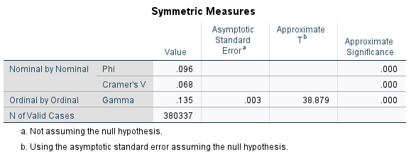
We can further explore the strength of the relationship with some symmetric measures. Symmetric measures don’t have an IV and a DV, but you should pick one based on the level of measurement. To use Gamma, both variables need to be ordinal. If one is nominal, just use the Phi or Cramer’s V. Phi will be identical to the Cramer’s V if you have a 2X2 table. If you don’t have a 2X2 table (like in our example), use the Cramer’s V. Here, we see a Cramer’s V of 0.068. You can use the following rough guidelines for interpreting both the Phi and the Cramer’s V

• ~0.10 weak relationship
• ~0.30 medium relationship
• ~0.50+ strong relationship

Our Cramer’s V here isn’t even up to 0.10, further confirming that the relationship between educational attendance and the number of bedrooms in your house is very weak.

When interpreting your results and presenting them in a paper, always make sure to make a nicer table than what SPSS provides and interpret both the forest and the trees. The forest is the big picture–in our case, there is a statistically significant relationship between where (and whether) someone attended school in the past 5 years and how many bedrooms they have (Χ²=3,511.860, df=8, p<0.001), however the relationship is weak (Lambda=0.022; Cramer’s V=0.068). The trees are all the little details, such as the differences I discussed above when looking at the initial table.

A nice looking table should always involve the following:

• Percentages going down the columns. Sometimes you might include the observed values, but they are not necessary and can overly clutter the table. Do not include the expected values.
• Properly labeled columns and rows
• A good title with the data named in parenthesis with the year (Canadian Census 2016) and typically we present the title as row by column (or DV by IV).
• Minimize the use of lines between cells
• Line up values at the decimal place
• Include the chi-square value, degrees of freedom, p-value and measures of association (lambda, gamma, phi, cramer’s-v, etc.) as a footnote to the table
• Make sure all fonts match within the table and to the rest of the paper; black ink
• Single space the text and remove any weird spacing issues

Well, doesn’t that look nice.